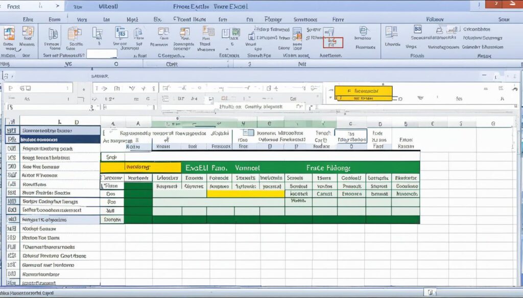
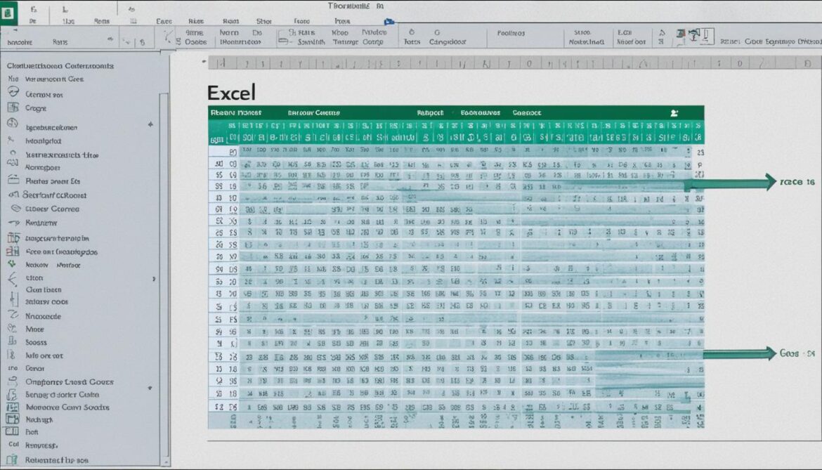
Freezing rows in Excel is a handy feature that allows you to keep certain rows, such as header cells, visible as you scroll through your spreadsheet. Whether you’re working with large amounts of data or need to reference important information while navigating your worksheet, freezing rows can make your life easier. In this guide, we’ll show you how to freeze rows in Excel and provide additional tips and tricks for working with frozen panes.
Key Takeaways:
- Freezing rows in Excel keeps specific rows visible as you scroll.
- To freeze a row, select the row below the one(s) you want to freeze, go to the View tab, and choose Freeze Panes.
- Excel also allows you to freeze columns, keeping them visible while scrolling horizontally.
- If you only need to freeze the first row or column, Excel provides specific options for that.
- You can easily unfreeze panes in Excel to restore normal scrolling behavior.
How to Freeze Rows in Excel
To freeze specific rows in Excel and keep them visible while scrolling through your spreadsheet, follow these simple steps:
- Select the row directly below the row(s) you want to freeze.
- Go to the View tab in the Excel ribbon.
- Click on the Freeze Panes option.
- Choose “Freeze Panes” from the dropdown menu.
By doing this, you lock the selected rows in place, allowing you to scroll vertically while keeping the frozen rows visible at the top.
Freezing the top row is especially useful when working with headers that need to remain visible. This feature ensures that you can always see the column names or other important information as you navigate through your spreadsheet.
Here is an example table to illustrate how freezing rows works in Excel:
| Name | Age | Occupation |
|---|---|---|
| John | 25 | Engineer |
| Sarah | 32 | Teacher |
| Michael | 41 | Accountant |
In this table, let’s say we want to freeze the top row which contains the column headers (Name, Age, Occupation). By following the steps mentioned earlier, we can freeze the top row and keep it visible as we scroll down the table.
Now, when we scroll vertically through the table, the frozen row stays at the top, providing a constant reference to the column names:
| Name | Age | Occupation |
|---|---|---|
| John | 25 | Engineer |
| Sarah | 32 | Teacher |
| Michael | 41 | Accountant |
| Emily | 29 | Doctor |
| David | 36 | Lawyer |
| Lisa | 27 | Marketing Manager |
As you can see, the frozen row (Name, Age, Occupation) remains visible at the top, even when scrolling further down the table.
How to Freeze Columns in Excel
In addition to freezing rows, you can also freeze columns in Excel. This feature is especially useful when dealing with wide spreadsheets and the need to keep specific columns visible at all times.
To freeze columns in Excel, follow these simple steps:
- Select the column to the right of the column(s) you want to freeze.
- Go to the View tab in Excel.
- Click on “Freeze Panes.”
By freezing columns, you can scroll horizontally in your spreadsheet while keeping the frozen columns visible on the left side. This creates a convenient window into your data, allowing you to focus on relevant information without losing context.
Example:
Let’s say you have a sales spreadsheet with multiple columns representing various product categories. You want to scroll through the data horizontally while keeping the “Product Name” column visible at all times. By freezing the “Product Name” column, you can easily navigate through the rest of the spreadsheet without losing sight of the product names.
Here’s a visual representation of how freezing columns works in Excel:
| Product Name | Category | Price | Quantity | Total |
|---|---|---|---|---|
| Product A | Category A | $10 | 5 | $50 |
| Product B | Category B | $20 | 3 | $60 |
| Product C | Category A | $15 | 8 | $120 |
As you scroll horizontally, the “Product Name” column remains fixed to the left side of the spreadsheet, providing constant visibility and easy reference.
By following these simple steps, you can effectively freeze columns in Excel and unlock the full potential of your spreadsheet organization and analysis.
Freezing the First Row or Column
If you only need to freeze the first row or column in your worksheet, Excel provides options for that as well. This feature comes in handy when you want to keep important information visible while scrolling through your data.
Freezing the Top Row
To freeze the top row, follow these steps:
- Go to the View tab.
- Click on Freeze Panes.
- Choose Freeze Top Row.
This will ensure that the top row remains in sight while you navigate through the rest of your worksheet.
Freezing the First Column
If you need to freeze the first column, here’s what you should do:
- Select any cell in the first column.
- Go to the View tab.
- Click on Freeze Panes.
- Choose Freeze First Column.
By doing this, the first column will stay in place even when you scroll horizontally through your spreadsheet.
This image demonstrates the process of freezing the first row or column in Excel, making it easier to reference critical information while working with large datasets.
Unfreezing Panes in Excel
If you have previously frozen panes in Excel and need to change your view options or remove the frozen panes, you can easily unfreeze them. This allows you to restore the normal scrolling behavior in your spreadsheet. Here’s how to unfreeze rows or columns:
- Go to the View tab at the top of the Excel window.
- Click on Freeze Panes in the Window group.
- Choose Unfreeze Panes from the dropdown menu.
By selecting “Unfreeze Panes,” Excel will remove the frozen panes and restore the ability to scroll freely through your spreadsheet. You can now navigate your data without the previously locked rows or columns.
Remember to save your Excel workbook after making any desired changes to your view options.
Unfreezing panes in Excel allows you to regain full control and flexibility in navigating your spreadsheet. Whether you need to adjust your view, modify locked rows or columns, or analyze data in a different context, Excel’s unfreeze panes feature gives you the freedom to customize your experience.
Other View Options in Excel
Excel offers additional view options to make it easier to compare and work with large worksheets. These features allow you to customize your workspace based on your specific needs. Two useful options to consider are opening a new window for your workbook and splitting a worksheet into separate panes.
Comparing Worksheets Side by Side
If you want to compare different worksheets side by side, Excel provides a convenient option to open a new window for your workbook. This allows you to view multiple worksheets simultaneously. To open a new window, follow these steps:
- Go to the View tab.
- Click on New Window.
- Arrange the windows accordingly to compare the desired worksheets.
This feature is beneficial when you need to analyze data across multiple sheets or refer to specific information while working on another worksheet. It enables a more efficient workflow, saving you time and effort.
Splitting a Worksheet into Separate Panes
In addition to opening a new window, Excel allows you to split a worksheet into separate panes. This feature is especially useful when you want to view different sections of the same worksheet simultaneously. Follow these steps to split a worksheet:
- Select the cell where you want to split the worksheet.
- Go to the View tab.
- Click on Split.
- Adjust the dividers as needed to create the desired pane sizes.
By splitting a worksheet, you can easily compare data within the same sheet, making it simpler to identify patterns, analyze trends, and make informed decisions based on the information at hand.
These view options in Excel provide flexibility and convenience, enhancing your ability to work with complex worksheets efficiently. Whether you need to compare different worksheets side by side or view different sections of a worksheet simultaneously, these features empower you to optimize your workflow and make the most of Excel’s capabilities.
Challenge: Comparing Data in Excel
To practice freezing and comparing data in Excel, you can try a challenge. Open a practice workbook that contains a lot of sales data. Freeze the first column and use the horizontal scroll bar to look at sales from a different year. Then, unfreeze the first column and split the worksheet into multiple panes to compare data for similar months from different years. This will help you understand how to manipulate frozen panes to analyze data effectively.
Here’s how you can perform this challenge:
- Open your Excel workbook that contains your sales data.
- Select the first column by clicking on the column header.
- Go to the View tab and click on the Freeze Panes button.
- Choose Freeze First Column from the dropdown menu.
- Scroll horizontally using the scroll bar to view sales data from different years while keeping the first column frozen.
- Unfreeze the first column by going back to the View tab and clicking on the Freeze Panes button.
- Choose Unfreeze Panes from the dropdown menu to restore normal scrolling.
- Select a cell where you want to split the worksheet into multiple panes.
- Go to the View tab and click on the Split button.
- Adjust the dividers as needed to compare data for similar months from different years.
By completing this challenge, you’ll gain hands-on experience with freezing and comparing data in Excel, allowing you to make informed decisions and spot trends more easily.

Conclusion
Freezing rows and columns in Excel is a powerful feature that allows you to keep important information visible while scrolling through large worksheets. This helps you stay organized and improves your efficiency when working with data. Whether you need to freeze a row, freeze a column, or compare data using frozen panes, Excel provides a range of options to meet your needs.
By freezing rows, you can easily reference essential information, such as header cells, while navigating through your spreadsheet. This feature is particularly handy when dealing with extensive data sets and complex worksheets.
To become a master of Excel spreadsheets, don’t hesitate to experiment with these freezing features. Take advantage of the ability to freeze rows, columns, and panes to customize your view and enhance your data analysis capabilities. With Excel’s comprehensive toolkit, you can confidently tackle any data-related task with ease.
FAQ
How do I freeze rows in Excel?
To freeze rows in Excel, select the row below the row(s) you want to freeze, go to the View tab, and choose Freeze Panes. This will lock the selected rows in place, allowing you to scroll through the spreadsheet while keeping the frozen rows visible at the top.
Can I freeze columns in Excel?
Yes, you can freeze columns in Excel. To freeze columns, select the column to the right of the column(s) you want to freeze, go to the View tab, and choose Freeze Panes. This will lock the selected columns in place, allowing you to scroll horizontally while keeping the frozen columns visible on the left side of the spreadsheet.
How do I freeze the top row in Excel?
To freeze the top row, go to the View tab, click Freeze Panes, and choose Freeze Top Row. This will keep the top row visible while you scroll through the rest of the worksheet.
How do I freeze the first column in Excel?
To freeze the first column, select a cell in the first column, go to the View tab, click Freeze Panes, and choose Freeze First Column. This will lock the first column in place while you navigate through the rest of the spreadsheet.
How can I unfreeze rows or columns in Excel?
To unfreeze rows or columns, go to the View tab, click Freeze Panes, and choose Unfreeze Panes. This will restore the normal scrolling behavior in your spreadsheet.
What are other view options in Excel?
Excel offers additional view options such as opening a new window for your workbook to compare different worksheets side by side. You can also split a worksheet into separate panes to view different sections simultaneously.
How can I compare data in Excel using frozen panes?
To compare data in Excel, you can freeze the first column and use the horizontal scroll bar to look at sales from a different year. You can also split the worksheet into multiple panes to compare data for similar months from different years.


