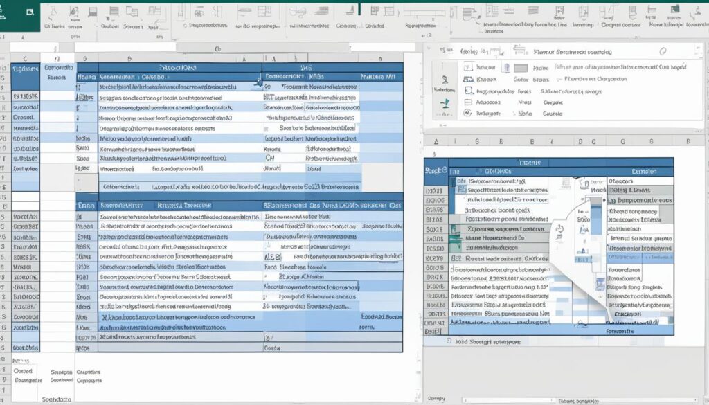
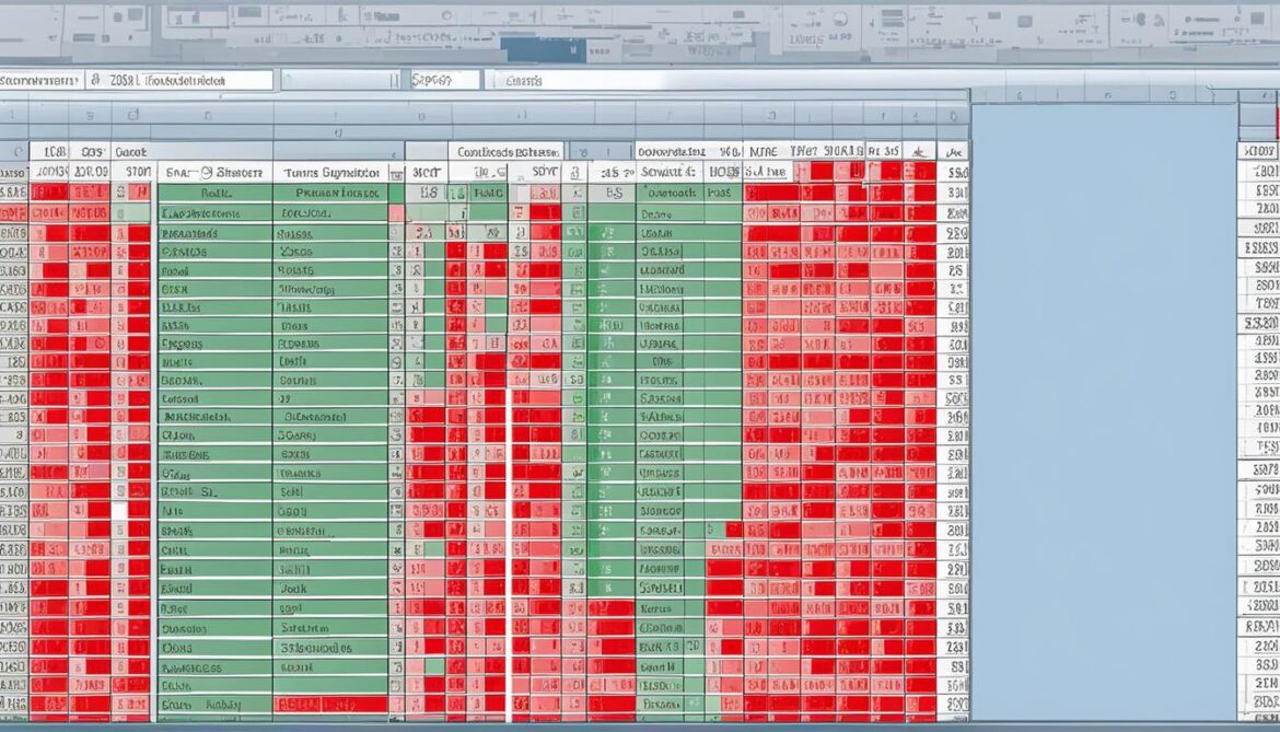
With the ever-increasing complexity and volume of data in today’s spreadsheets, it can be a daunting task to manually identify and remove duplicate values in Excel. However, ignoring duplicates can lead to inaccurate data analysis and flawed insights. To ensure the accuracy of your analysis, it is crucial to de-duplicate your data before diving into your Excel sheet.
Key Takeaways:
- Identifying and removing duplicates is key to accurate data analysis in Excel.
- Manually spotting duplicates in large datasets is virtually impossible.
- De-duplicating data ensures the reliability and integrity of your analysis.
- Conditional Formatting in Excel is an easy and efficient method to identify duplicate values.
- Using Excel’s built-in “Remove Duplicates” feature can quickly eliminate duplicate rows.
Simple and Easy Method to Find Duplicates in Excel
A simple and easy method to find duplicates in Excel is to use Conditional Formatting. This feature allows you to highlight duplicate values within a selected data range, making it effortless to identify and manage duplicate entries. By applying the “Highlight Cell Rules” option under the Conditional Formatting menu, you can quickly spot and address duplicate values in any column.
Steps to Identify Duplicate Values in Excel:
- Select the data range in which you want to identify duplicate values.
- Navigate to the “Home” tab in the Excel ribbon.
- Click on the “Conditional Formatting” button.
- Choose the “Highlight Cell Rules” option.
- Select the duplicate values condition, such as “Duplicate Values…” or “Duplicate Values with Format…”
- Customize the formatting options if desired.
- Click “OK” to apply the formatting.
With Conditional Formatting, you can visually distinguish duplicate values from unique ones, allowing you to identify any recurring data patterns or errors in your Excel sheet. This method is particularly useful when working with large datasets, as it offers a quick and efficient solution to identify duplicate values without the need for complex formulas or manual inspection.
To further aid your understanding, take a look at the comparison table below:
| Data | Duplicate? |
|---|---|
| Apple | No |
| Orange | No |
| Apple | Yes |
| Banana | No |
| Apple | Yes |
As illustrated in the table above, the Conditional Formatting feature allows you to quickly identify duplicate values in the “Data” column, marking them as “Yes” in the “Duplicate?” column. This visual representation makes it effortless to locate and manage duplicate values in your Excel sheets.
Using Conditional Formatting to Find Partial Matches
If you want to identify and highlight partial matches or values similar to duplicates in Excel, you can easily achieve this using the powerful feature called Conditional Formatting. This feature allows you to customize the formatting of specific cells based on certain conditions, such as partial matches. By utilizing the “Text That Contains” setting under Conditional Formatting, you can effectively highlight partial matches in your Excel spreadsheet.
Here’s how you can use Conditional Formatting to highlight duplicates in Excel:
- Select the range of cells where you want to identify partial matches or potential duplicates.
- Go to the Home tab and click on the Conditional Formatting dropdown menu.
- Choose the “Highlight Cells Rules” option.
- Select “Text That Contains” from the list.
- In the dialog box that appears, enter the specific text or characters that represent the partial matches you want to identify. For example, if you want to find all values that contain the word “duplicate,” enter “duplicate” in the text box.
- Choose the formatting style you prefer for highlighting the partial matches. This could be a different font color, background color, or any other formatting option available in Excel.
- Click on the “OK” button to apply the Conditional Formatting rule.
Once you’ve applied the Conditional Formatting rule, Excel will automatically highlight all cells that contain the specified text or characters. This makes it easier to identify and manage partial matches or potential duplicates within your spreadsheet.
Example:
- Suppose you have a column of product names in your Excel sheet.
- By applying Conditional Formatting with the “Text That Contains” rule and entering “duplicate” as the text, Excel will highlight all cells that contain the word “duplicate” in the product names column.
- This allows you to quickly identify any partial matches or potential duplicates in your product names.
By using Conditional Formatting in Excel, you can efficiently highlight partial matches and manage potential duplicates in your spreadsheet. This powerful feature saves you valuable time and ensures the accuracy of your data analysis.
Removing Duplicates in Excel
When working with large datasets in Excel, it’s common to encounter duplicate values that can skew your analysis or cause inconsistencies in your data. Fortunately, Excel provides a built-in feature called “Remove Duplicates” that allows you to quickly and effortlessly eliminate duplicate rows or entries from your Excel sheet.
To access the “Remove Duplicates” feature, navigate to the Data Tab in the Excel ribbon. Look for the Data Tools group, where you’ll find the option to remove duplicates. Click on this button to initiate the process.
Before removing duplicates, it’s crucial to select the data range that you want to de-duplicate. This can be a single column, multiple columns, or the entire worksheet if needed. Excel will analyze the selected data range and identify any duplicate rows.
Once you have selected the desired range, click on the “Remove Duplicates” button. Excel will present you with a prompt that allows you to choose which columns to consider when determining duplicates. You can select specific columns or choose to evaluate all columns for duplicates.
After making your selections, click the “OK” button, and Excel will remove the duplicate rows from your dataset. The remaining entries will be unique, helping you maintain data integrity and accuracy for further analysis.
Example:
Let’s say you have a worksheet containing a list of customer names and email addresses. However, due to manual data entry or other factors, some customers’ information may have been duplicated. To remove these duplicates, follow the steps outlined above.
| Customer Name | Email Address |
|---|---|
| John Smith | [email protected] |
| Jane Doe | [email protected] |
| John Smith | [email protected] |
| Customer Name | Email Address |
|---|---|
| John Smith | [email protected] |
| Jane Doe | [email protected] |
After removing duplicates, your table will look like this:
| Customer Name | Email Address |
|---|---|
| John Smith | [email protected] |
| Jane Doe | [email protected] |
As you can see, the duplicate entry for John Smith and [email protected] has been removed, leaving only the unique values in the dataset.
Comparing Two Excel Sheets for Duplicates
If you need to compare two Excel sheets for duplicates, there are a few different methods you can use. One common approach is to use Conditional Formatting in Excel. By selecting the range in the first sheet, you can use a formula to determine which cells to format and highlight duplicate values. Another method is to use Excel’s “Remove Duplicates” feature, which allows you to compare and remove duplicate data from multiple sheets.
When using Conditional Formatting, start by selecting the data range in the first sheet that you want to compare with the second sheet. Then, go to the “Home” tab and click on “Conditional Formatting” in the “Styles” group. Choose the “Highlight Cells Rules” option and select “Duplicate Values.” Customize the formatting style as needed, and Excel will highlight the duplicate values across the two sheets.
If you prefer to use the “Remove Duplicates” feature, begin by selecting the range in the first sheet that contains the data you want to compare. Then, go to the “Data” tab and click on the “Remove Duplicates” button in the “Data Tools” group. Excel will prompt you to select the columns to compare, and it will remove any duplicate rows based on your selection.
Both methods provide effective ways to identify and manage duplicates when comparing two Excel sheets. Choose the option that best fits your specific needs and preferences.

| Methods | Advantages | Disadvantages |
|---|---|---|
| Conditional Formatting | Quick and visual identification of duplicate values | Does not automatically remove duplicates |
| Remove Duplicates feature | Easy and efficient removal of duplicate rows | Permanent removal of duplicates |
By utilizing these methods, you can effectively compare two Excel sheets for duplicates and ensure the integrity of your data. Whether you choose to highlight the duplicates or remove them entirely, Excel provides the necessary tools to streamline your data analysis and management processes.
Using Excel Formulas to Find Duplicate Data
Excel formulas are a powerful tool that can help you identify and handle duplicate data in your spreadsheets. By using functions like VLOOKUP, INDEX, MATCH, and COUNTIF, you can easily locate duplicate values across multiple sheets or within a single sheet. These formulas can be complemented by conditional formatting, allowing you to highlight duplicate values for better visibility and analysis.
For instance, let’s say you have a dataset with customer names and email addresses on one sheet, and you want to find any duplicate email addresses. You can use the COUNTIF function to check how many times each email address appears in the range. If the count is greater than 1, that means it is a duplicate. By combining this formula with conditional formatting, you can highlight these duplicates, making it easier to take necessary actions.
Additionally, Excel formulas can be used to remove duplicate data from your sheets. By applying a combination of functions and filters, you can efficiently manage and eliminate duplicate values. For example, the INDEX and MATCH functions can help you identify and remove duplicate rows or columns in your dataset.
By leveraging the power of Excel formulas, you can streamline your data analysis process and ensure the accuracy and integrity of your spreadsheets. Whether you need to highlight duplicate values, compare data across sheets, or remove duplicates, Excel formulas provide a versatile and efficient solution. With a deeper understanding of these formulas, you can enhance your productivity and make the most out of Excel’s data management capabilities.
FAQ
How can I find duplicates in Excel?
A simple and easy method to find duplicates in Excel is to use Conditional Formatting. Select the data range where you want to spot the duplicate values and choose the option “Highlight Cell Rules” under the Conditional Formatting menu.
How do I identify partial matches or similar duplicates in Excel?
You can use Conditional Formatting in Excel to identify partial matches. By using the “Text That Contains” setting under Conditional Formatting, you can pick partial matches to be highlighted in Excel, making it easier to identify and manage duplicates.
How can I remove duplicates in Excel?
To remove duplicates in Excel, you can use the built-in “Remove Duplicates” feature. This feature can be found in the Data Tab under the Data Tools group.
How can I compare two Excel sheets for duplicates?
There are a few different methods you can use to compare two Excel sheets for duplicates. One common approach is to use Conditional Formatting in Excel to highlight duplicate values. Another method is to use Excel’s “Remove Duplicates” feature to compare and remove duplicate data from multiple sheets.
Can I use Excel formulas to find and highlight duplicate data?
Yes, Excel formulas can be used to find and highlight duplicate data in Excel sheets. Functions like VLOOKUP, INDEX, MATCH, and COUNTIF can be combined with conditional formatting to identify duplicates across sheets or within a sheet.


